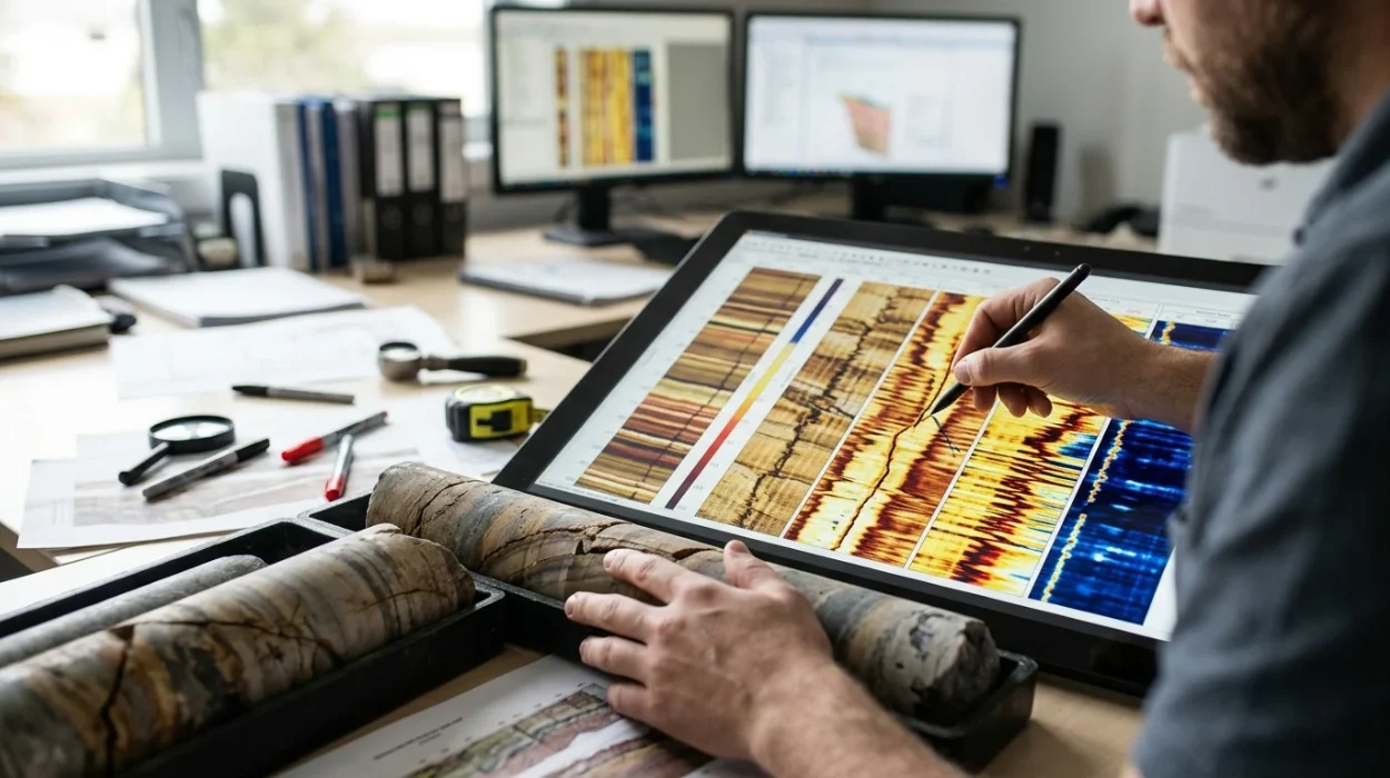
Borehole image log processing and interpretation transform raw downhole sensor measurements into oriented, high-resolution structural and sedimentological models of the subsurface. Petrophysicists, structural geologists, and reservoir engineers use these processed images to resolve thin beds, characterise natural fracture networks, and determine in-situ stress orientations with millimetre-scale vertical resolution. Accurate geological evaluation depends on strict adherence to acquisition quality control, systematic speed correction, dynamic image normalisation, and standardised feature picking across both wireline and logging-while-drilling datasets.
Subsurface asset teams rely on high-definition borehole imagery when conventional triple-combo wireline logs lack the vertical resolution required to detect sub-seismic faults or centimetre-scale stratigraphic laminations. Understanding why borehole image processing matters in oil and gas well log analysis establishes the foundational link between raw downhole electrical or acoustic signals and commercial reservoir characterisation. Moving from raw field data to a calibrated geological model requires evaluating distinct processing methodologies, tool physics, and workforce competency frameworks.
What Are the Core Stages of Borehole Image Log Processing?
Borehole image log processing converts raw downhole array signals into oriented, depth-matched static and dynamic visualisations through six sequential steps: data loading, image log quality control, accelerometer speed correction, pad-to-pad normalisation, borehole orientation calculation, and amplitude histogram equalisation.
Raw acquisition files arrive from the wellsite in standard formats such as DLIS or LIS, containing multi-pad microresistivity curves or ultrasonic transit-time and amplitude waveforms alongside triaxial accelerometer and magnetometer channels. Each processing stage eliminates mechanical, electrical, or borehole-induced artefacts before a geologist assigns structural dips or facies classifications. Skipping or miscalibrating any intermediate step propagates geometric distortion directly into the reservoir fracture model.
1. Image Log Quality Control and Pre-Processing
Image log quality control begins with verifying tool orientation channels against directional survey records to confirm magnetic declination and grid convergence corrections. Processors inspect raw pad button curves for dead electrodes, saturated signals, mudcake stand-off, and telemetry dropouts. If tool eccentering exceeds 0.5 inches or magnetic interference from bottom-hole assembly components distorts magnetometer readings by more than 3 degrees, the dataset requires corrective filtering or flagging prior to structural dip computation.
2. Accelerometer Speed Correction and Depth Alignment
Downhole tools experience irregular motion, including stick-slip and cable stretch, even when surface winch speed remains constant. Processors integrate triaxial Z-axis accelerometer data to calculate true instantaneous tool velocity and shift individual button measurements onto a uniform depth grid. Without accurate speed correction, horizontal bedding planes appear stretched or compressed, creating false apparent dips exceeding 10 to 15 degrees across short intervals.
3. Pad-to-Pad Calibration and Image Normalisation
Microresistivity imaging tools employ multiple articulated pads pressed against the borehole wall, with each pad carrying rows of button electrodes that exhibit slight gain and offset variations. Static normalisation applies a single global gain and offset across the entire logged interval to preserve absolute formation resistivity contrasts, allowing geologists to distinguish shale baselines from high-resistivity carbonate or cemented intervals. Dynamic normalisation applies a sliding depth window—typically 1 to 2 metres—to enhance local contrast, revealing subtle cross-bedding, bioturbation, and hairline fractures inside otherwise homogeneous formations.
How Do Microresistivity and Acoustic Image Processing Workflows Differ?
Microresistivity tools like FMI and OBMI measure formation electrical impedance through conductive or oil-based muds, whereas acoustic ultrasonic tools measure borehole wall reflection amplitude and two-way travel time, requiring distinct processing algorithms for mud attenuation, pad coverage, and borehole geometry.
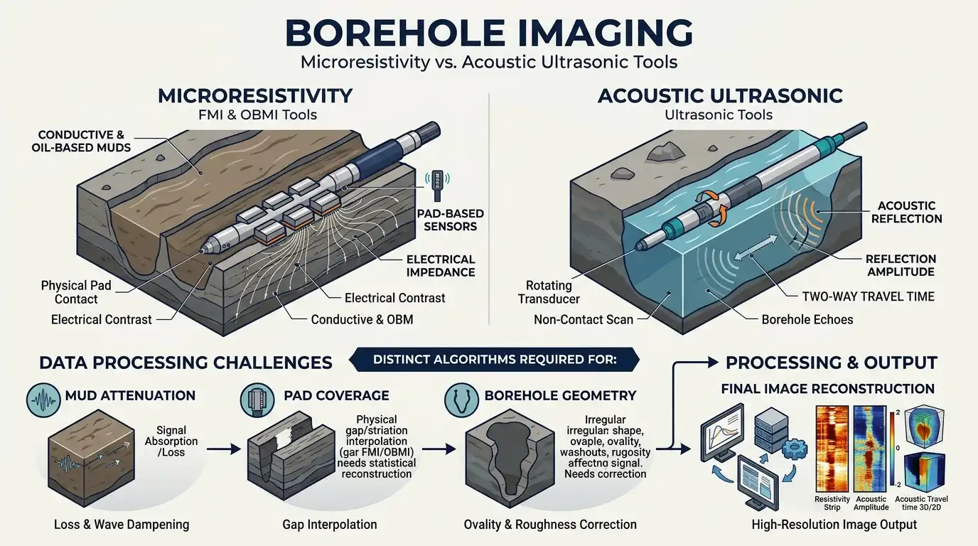
Selecting the appropriate processing workflow and interpretation methodology depends directly on the mud system and physical measurement principle deployed in the well. Water-based mud systems support high-resolution galvanic microresistivity measurements, while oil-based mud systems require capacitive coupling or acoustic pulse-echo physics. Geoscientists and technical training managers must align interpretation protocols with the exact tool family used in their target basins.
Evaluation Attribute | Water-Based Mud Microresistivity (FMI) | Oil-Based Mud Microresistivity (OBMI) | Ultrasonic Acoustic Imaging (UBI / CBIL) |
Physical Measurement | Direct galvanic electrical current injection | Capacitive/inductive impedance coupling | High-frequency ultrasonic pulse-echo (250–500 kHz) |
Vertical Resolution | 5 mm (0.2 inches) | 12–15 mm (0.5 inches) | 5–10 mm (0.2–0.4 inches) |
Azimuthal Borehole Coverage | ~80% in an 8.5-inch borehole | ~32%–45% in an 8.5-inch borehole | 100% continuous 360-degree coverage |
Primary Processing Artefacts | Pad lift-off, dead buttons, stick-slip | High-frequency noise, mud-film stand-off | Eccentering, heavy mud attenuation, breakout scatter |
Optimal Geological Application | Thin-bed sand-shale counts, fine fracture aperture | Structural dip, macro-fracture orientation | Borehole breakout stress analysis, vuggy carbonate mapping |
FMI Interpretation in Conductive Mud Systems
FMI interpretation (Fullbore Formation MicroImager) leverages dense arrays of 192 micro-electrodes across four pads and four flaps to achieve 5-millimetre vertical resolution. Because conductive water-based mud provides direct electrical contact between the buttons and the formation, conductive drilling mud invades open natural fractures and creates sharp, dark sinusoidal traces on the processed image. Processing workflows for FMI datasets prioritise inter-pad button equalisation and dead-button interpolation to prevent vertical striping from obscuring low-angle sedimentary structures.
OBMI Interpretation in Non-Conductive Mud Systems
OBMI interpretation (Oil-Base MicroImager) addresses the electrical insulation barrier created by non-conductive oil-based or synthetic-based drilling fluids. The tool injects alternating current into the formation and measures potential differences across button pairs, resulting in lower azimuthal coverage (roughly 32% in an 8.5-inch hole) and wider blank gaps between pads than FMI logs. Processors apply aggressive dynamic normalisation and dip-interpolation algorithms across the blank pad gaps to reconstruct continuous sinusoidal planes for structural analysis.
Acoustic Ultrasonic Image Processing
Acoustic borehole imagers emit rotating ultrasonic pulses from a central transducer and record both reflected wave amplitude and two-way travel time across a full 360-degree circumference. Processing acoustic logs requires borehole radius correction to remove transit-time ovalisation caused by tool eccentering, alongside mud-slowness calibration for high-density drilling fluids. Unlike electrical logs, acoustic travel-time images directly quantify borehole wall geometry, making them the benchmark dataset for measuring borehole breakouts and drilling-induced tensile fractures.
How Are Structural and Sedimentological Features Interpreted from Processed Images?
Geologists interpret processed borehole images by fitting oriented sinusoidal curves to planar features across 360-degree unwrapped plots, classifying structural dips, natural fractures, and borehole breakouts before integrating them with core and open-hole petrophysical logs.
On an unwrapped borehole image oriented to True North, any planar geological feature intersecting the cylindrical wellbore appears as a sinusoid. The amplitude of the sinusoid reflects the true dip angle relative to the borehole axis, while the trough of the curve indicates the dip azimuth. Accurate interpretation requires strict classification rules so that drilling-induced artefacts are never mistaken for natural permeability pathways.
Fracture Identification and Aperture Quantification
Fracture identification distinguishes open natural fractures, healed mineralised fractures, and drilling-induced tensile fractures based on sinusoidal continuity, dip azimuth, and electrical conductivity contrast. In water-based mud microresistivity images, open fractures appear as continuous, dark (conductive) sinusoids that cut across primary bedding planes, whereas healed calcite- or quartz-filled fractures appear as bright (resistive) sinusoids. Once an open fracture is picked, interpreters apply Luthi-Souhaite calibration equations using flushed-zone resistivity ($R_{xo}$) and mud resistivity ($R_m$) to estimate hydraulic fracture aperture in millimetres.
Structural Analysis and Fold-Fault Zonation
Systematic structural analysis involves filtering out tectonic tilt from depositional cross-bedding using stereonet projections, tadpole plots, and cumulative dip vectors. Abrupt shifts in dip magnitude or azimuth across a narrow depth interval indicate fault drag zones, unconformities, or angular fault planes. Geoscientists separate structural dips into coherent stratigraphic domains, enabling reservoir engineers to update seismic horizon depth conversions and refine fault-seal integrity models.
Geomechanical Stress Profiling
Interpreters identify borehole breakouts as pairs of wide, poorly resolved dark vertical bands separated by 180 degrees on microresistivity images, or as deep transit-time enlargements on acoustic caliper logs. Breakouts form parallel to the minimum horizontal stress direction ($S_{hmin}$), while narrow, vertical drilling-induced tensile fractures form at 90 degrees to breakouts, indicating the maximum horizontal stress azimuth ($S_{Hmax}$). Quantifying stress orientation across reservoir intervals directly guides horizontal well trajectory planning and hydraulic fracturing stage placement.
Which Learning Approaches Best Close Enterprise Workforce Skill Gaps in Image Log Analysis?
Organisations close borehole image interpretation skill gaps by comparing self-paced software tutorials, vendor-specific tool workshops, and structured corporate training programs against technical competency KPIs, turnaround time targets, and subsurface risk reduction.
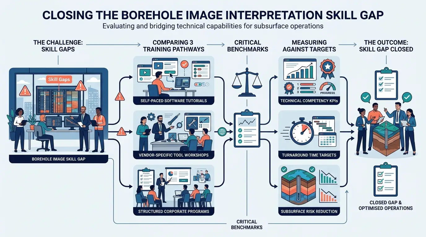
Upstream operating companies and service providers frequently face an acute talent bottleneck: fewer than 25% of early-career geoscientists possess hands-on proficiency in raw image log quality control and multi-tool structural picking. Relying exclusively on external service company interpretations introduces multi-week project delays and creates a disconnect between image log picks and local basin stratigraphy. HR directors and subsurface technical managers must evaluate distinct training delivery models to build internal analytical capability.
Training Delivery Model | Primary Learning Focus | Typical Duration | Operational Impact on Asset Teams | Key Limitation |
Vendor Software Tutorials | User-interface navigation and button-clicking workflows | 2–3 days | Accelerates basic workstation familiarity | Lacks geological QC principles and multi-tool physics comparison |
Academic Short Courses | Theoretical sedimentology and outcrop analogues | 4–5 days | Builds strong conceptual facies recognition | Omits real-world mud-system artefacts and raw DLIS speed correction |
Structured Corporate Technical Training | End-to-end QC, processing workflows, and multi-well reservoir integration | 5 days (instructor-led) | Reduces external consulting spend by 40%–60% and cuts interpretation cycle time | Requires dedicated pre-course dataset alignment |
Evaluating Technical Competency and Operational ROI
When HR teams and subsurface department heads compare training investments, measurable return on investment centres on three operational KPIs: interpretation turnaround time, reduction in non-productive drilling time (NPT), and external vendor expenditure. A single misidentified fracture corridor or uncalibrated structural dip in a horizontal appraisal well can misplace a completion stage, costing between $250,000 and $1.2 million in lost production or remedial workovers. Structured corporate training programs directly mitigate this exposure by standardising quality control checklists across petrophysics and geology teams.
Organizations ready to standardise their subsurface workflows and upskill multidisciplinary asset teams often evaluate comprehensive curricula such as Borehole Image Processing and Interpretation Training by Institute For Oil & Gas Training. Unlike generic software walkthroughs, structured corporate programs train geoscientists to audit vendor-processed deliverables, perform independent accelerometer speed corrections, and reconcile FMI, OBMI, and acoustic datasets within live reservoir modelling environments.
Selecting the Right Curriculum for Asset Team Maturity
Selecting an enterprise learning framework requires matching course depth to the existing skill distribution across junior, mid-level, and senior geoscientists. Technical managers should apply a structured evaluation framework before committing training budgets to ensure immediate workplace transfer.
Evaluation Criterion | Junior Geoscientist Cohort (0–3 Years) | Experienced Asset Team Cohort (4+ Years) |
Core Competency Gap | Basic sinusoid picking, tadpole plot reading, and tool physics fundamentals | Raw data QC auditing, complex fracture aperture modelling, and geomechanical stress integration |
Required Practical Lab Ratio | 60% guided interpretation exercises, 40% foundational theory | 75% multi-well troubleshooting labs (faulted/fractured reservoirs), 25% advanced algorithms |
Delivery Format | Blended instructor-led classroom with supervised workstation labs | Intensive workshop using company-specific well logs and regional structural analogues |
Post-Training Validation KPI | Independent completion of a single-well structural and facies zonation report | Reduction of vendor QC turnaround time by 50% and zero unflagged orientation errors |
Enrolling technical personnel in a dedicated Borehole Image Processing and Interpretation Training Course equips asset teams with repeatable workflows for raw data auditing, dynamic normalisation, and quantitative fracture evaluation. By embedding standardised interpretation protocols across exploration and development teams, organisations protect capital allocation decisions and maximise hydrocarbon recovery from structurally complex reservoirs.
Frequently Asked Questions
What is Oil & Gas Borehole Imaging and why is it used in formation evaluation?
Oil & Gas Borehole Imaging is a high-resolution downhole logging technique that generates 360-degree electrical or acoustic visualisations of the borehole wall. At the Institute For Oil & Gas Training, technical modules demonstrate how these microresistivity and ultrasonic image logs resolve thin beds, characterise natural fracture networks, and determine in-situ stress orientations far beyond the resolution of conventional open-hole logs.
How do microresistivity and acoustic borehole imaging tools differ?
Microresistivity tools measure variations in formation electrical conductivity using articulated pads pressed against the borehole wall, whereas acoustic ultrasonic tools measure the reflection amplitude and two-way travel time of high-frequency sound waves. Programmes in Oil & Gas Borehole Imaging delivered by the Institute For Oil & Gas Training train subsurface teams to select microresistivity imagers for high-resolution thin-bed analysis in conductive muds and acoustic televiewers for full 360-degree borehole geometry and breakout evaluation.
Which borehole imaging method works best in oil-based drilling muds?
Oil-based mud (OBM) microresistivity imagers and ultrasonic acoustic tools are specifically engineered to operate in non-conductive drilling fluids where standard galvanic electrical tools cannot pass current into the formation. Through practical Oil & Gas Borehole Imaging workshops at the Institute For Oil & Gas Training, geoscientists learn to process capacitive-coupling OBM logs and mitigate mud-attenuation artefacts in heavy synthetic fluids.
How are natural fractures identified on processed borehole image logs?
Interpreters identify open natural fractures by fitting oriented sinusoidal curves to continuous, dark conductive traces that cut across primary sedimentary bedding planes on unwrapped 360-degree plots. Curricula covering Oil & Gas Borehole Imaging at the Institute For Oil & Gas Training equip petrophysicists and structural geologists to distinguish conductive open fractures from resistive mineral-healed fractures and drilling-induced tensile fractures.
What role does quality control play in borehole image processing and interpretation?
Rigorous image log quality control (QC) eliminates tool stick-slip distortion, dead electrode striping, and magnetometer interference before structural dips or fracture apertures are calculated. The Institute For Oil & Gas Training incorporates standardised QC auditing workflows into its Oil & Gas Borehole Imaging courses so asset teams can verify accelerometer speed corrections and orientation accuracy prior to building reservoir models.
Related training courses
Acoustic Borehole Imaging Technologies Training Course
- Specialisation
- Oil & Gas Borehole Imaging
- Duration
- 5 days · 15 CPD hours
Borehole Image Analysis for In-Situ Stress Evaluation Training Course
- Specialisation
- Oil & Gas Borehole Imaging
- Duration
- 5 days · 15 CPD hours
Borehole Image Applications for Reservoir Characterization Training Course
- Specialisation
- Oil & Gas Borehole Imaging
- Duration
- 5 days · 15 CPD hours
More articles
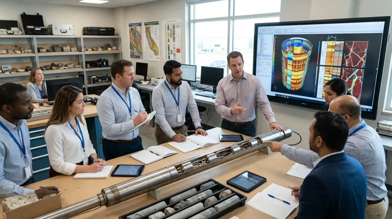
Electrical Borehole Imaging Technologies Training by Institute For Oil & Gas Training
Discover the curriculum, learning outcomes, and enrollment process for the Electrical Borehole Imaging Technologies Training Course.
Read article →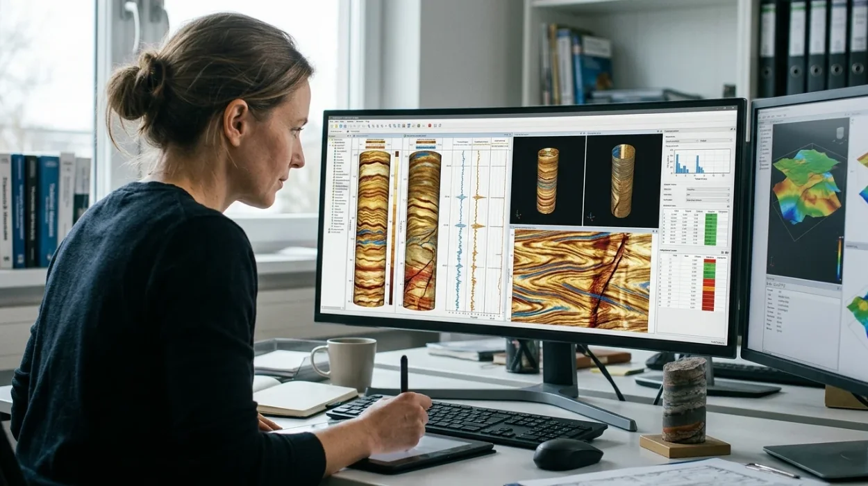
How to Evaluate Electrical Borehole Imaging Technologies and Their Applications in Formation Analysis
Master how to evaluate electrical borehole imaging technologies formation microimagers and resistivity logging tools for advanced subsurface analysis.
Read article →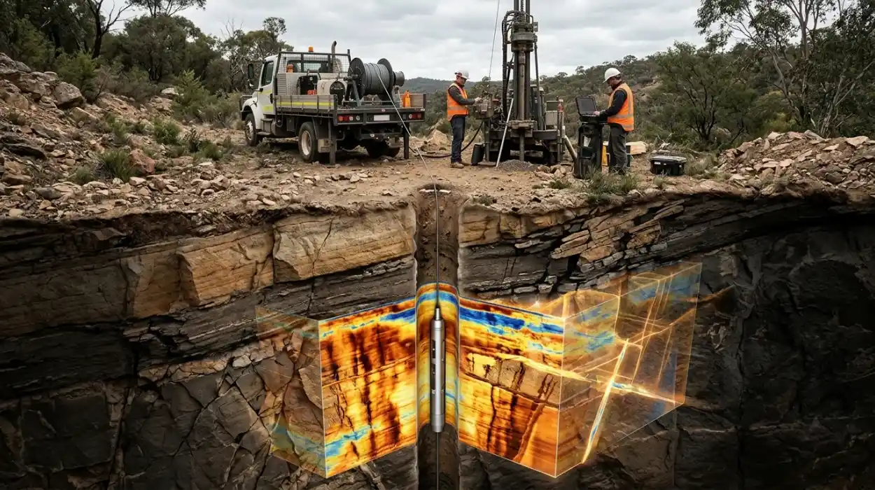
How Electrical Borehole Imaging Improves Subsurface Geological Understanding
Learn how electrical borehole imaging improves subsurface geological understanding and workforce competency through structured corporate technical training.
Read article →