How to Evaluate Production Forecasts and Decline Curves for Reliable Financial Analysis

Financial models in the upstream oil and gas sector rely directly on the accuracy of production volume projections. Evaluating production forecasts and decline curves allows financial analysts, investment managers, and corporate planners to convert complex subsurface reservoir data into reliable cash flow projections, asset valuations, and capital allocation frameworks.

Petroleum economists and corporate finance teams must understand Why Production Forecasting and Decline Curve Analysis Matter in Oil and Gas Financial Planning when assessing operational risk, debt capacity, and project return profiles. Production forecasting provides the baseline volume assumptions that dictate revenue recognition, depletion calculations, tax liabilities, and operating cost distribution over the lifecycle of an asset.

What Are the Core Components of Production Forecasting in Oil and Gas Financial Analysis?

Production forecasting relies on initial production rates, decline rate estimation, well performance history, type curves, and cumulative production limits to establish expected cash flows. These technical components convert raw subsurface flow dynamics into deterministic metrics required for capital budgeting and risk assessment.

Upstream financial valuation begins with the initial production rate, which measures the initial volume output of a well after completion and flowback. Financial analysts use this starting metric to establish the peak revenue period for short-term budget planning.

The baseline performance shifts as field development progresses. Engineers divide production profiles into distinct operational stages:

• Plateau phase: Represents the early period where production remains constant due to facility capacity limits or managed drawdowns.

• Decline phase: Marks the secondary period where continuous pressure depletion reduces overall flow rates over time.

To quantify this transition across undeveloped acreage, finance teams employ a type curve. A type curve represents an aggregated production profile created from historical well performance history across geologically similar analog wells. It establishes the baseline expectation for future drilling locations.

Accurate evaluation requires precise decline rate estimation. Analysts calculate the percentage loss in production over specified time intervals to forecast short-term cash flows. This calculation directly impacts the estimated ultimate recovery, which defines the total cumulative volume of hydrocarbons economically recoverable from a well or field before reaching its economic limit.

Understanding these subsurface flow indicators prevents capital misallocation. Upstream energy finance teams must translate reservoir depletion metrics directly into balance sheet projections and dynamic debt service coverage ratios.

How Do Exponential, Hyperbolic, and Harmonic Decline Curves Differ in Financial Modeling?

Exponential decline assumes a constant percentage drop, hyperbolic decline features a decreasing decline rate over time, and harmonic decline applies when fluid viscosity governs flow. Each mathematical model creates distinct long-term revenue trajectories, cash flow assumptions, and final asset valuation outcomes.

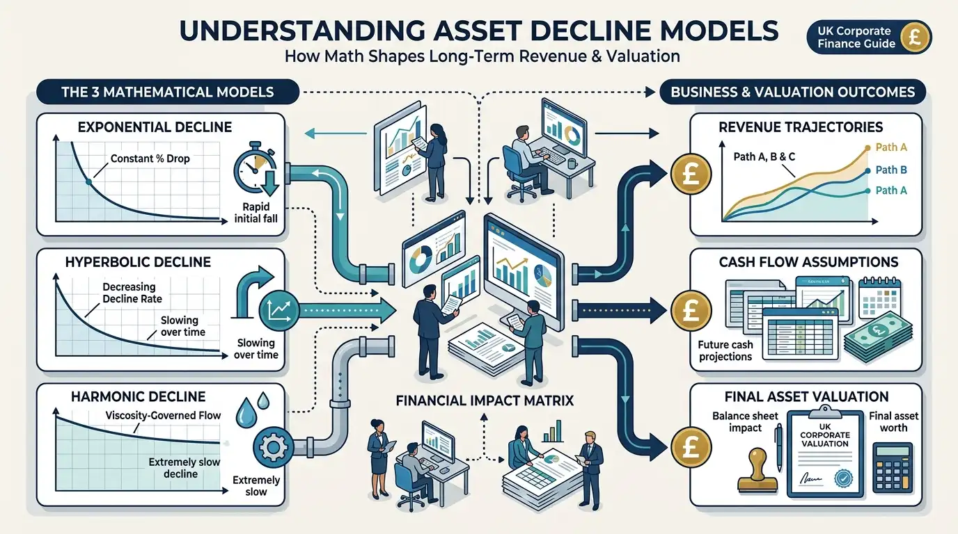
Arps decline equations provide the mathematical foundation for empirical decline curve analysis in petroleum economics. Financial modelers must select the correct mathematical decline model based on reservoir drive mechanisms, fluid characteristics, and extraction methodologies.

Selecting an incorrect curve type distorts cash flow expectations and leads to significant mispricing during asset acquisitions or impairment testing.

Exponential Decline

Exponential decline occurs when the fractional change in production rate per unit of time remains constant. The fractional decline rate ($D$) remains static throughout the well lifecycle.

This model applies primarily to single-phase fluid flow, highly depleted conventional reservoirs, or wells operating under constant back-pressure. In financial modeling, exponential decline delivers the most conservative revenue projections. It produces a steeper early drop in production, leading to shorter projected well lifespans and lower overall valuations.

Hyperbolic Decline

Hyperbolic decline occurs when the fractional decline rate decreases over time. The hyperbolic exponent ($b$-factor) ranges between zero and one in standard conventional reservoirs, though unconventional shale formations frequently exhibit initial $b$-factors greater than one.

Hyperbolic models capture the transient boundary-dominated flow common in low-permeability reservoirs. For financial analysts, hyperbolic curves project higher long-term tail production than exponential models. Overestimating the $b$-factor inflates ultimate recovery estimates and overstates long-term asset value.

Harmonic Decline

Harmonic decline represents a specific hyperbolic case where the $b$-factor equals exactly one. In this scenario, the fractional decline rate is directly proportional to the production rate itself.

Harmonic behavior occurs in gravity-drainage reservoirs, full water-drive systems, or high-viscosity crude operations. From a corporate finance perspective, harmonic curves generate the longest tail production profiles. This creates steady, long-term cash flows, but requires continuous operational expenditure monitoring to ensure the well remains above its economic limit.

What Comparative Evaluation Framework Determines the Reliability of a Production Forecast?

Evaluating forecast reliability requires assessing data density, historical match quality, geological analog consistency, and economic limit sensitivity. Comparing these analytical criteria across technical inputs isolates underlying subsurface risks and prevents systemic overestimation in financial models.

Finance professionals must rigorously audit production assumptions before incorporating them into acquisition models or corporate reserves reporting. Evaluating technical forecasts against structured benchmark criteria reveals structural bias and isolates operational vulnerabilities.

A robust evaluation framework demands cross-functional alignment between engineering data and financial systems. Upstream teams must continually test subsurface forecasts against historical accounting performance to verify that technical decline assumptions match real-world cash generation.

How Can Finance Teams Audit Decline Curve Analysis for Asset Valuation and Risk Management?

Finance teams audit decline curves by verifying historical well performance history, stress-testing decline rate estimation parameters, validating type curve normalization methods, and cross-referencing reserves classification standards. This technical verification process reduces investment risk and ensures regulatory compliance.

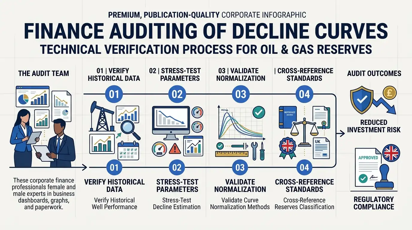
An effective financial audit converts raw decline metrics into audited capital figures. Corporate analysts must execute targeted audit steps across four main technical domains to validate underlying reserve values.

Step 1: Historical Well Performance Reconciliation

The audit begins by plotting historical monthly production volumes against projected decline curves on semi-logarithmic scales. Analysts check whether actual flow rates systematically underperform the initial model. Discrepancies point to mechanical downtime, unannounced shut-ins, artificial lift failures, or fundamentally flawed reservoir pressure assumptions.

Step 2: $b$-Factor and Terminal Decline Validation

Analysts must inspect the long-term decline mechanics within hyperbolic models. Unconventional wells modeled with high initial $b$-factors ($b > 1.0$) must transition to a flat exponential decline rate—known as the terminal decline rate ($D_{lim}$)—once boundary-dominated flow stabilizes. Failing to apply a terminal decline rate between 5% and 8% creates unrealistically high long-term production, artificially inflating the net present value of the asset.

Step 3: Type Curve Normalization Verification

When evaluating undeveloped locations, financial auditors must verify how technical teams normalized the underlying type curve. Production profiles normalized solely on completed lateral length may ignore key variables like completion fluid intensity, stage spacing, or cluster density. Finance teams require normalized type curves that mirror actual planned capital expenditure programs.

Step 4: Reserve Classification Alignment Check

Finally, production forecasts must align with formal reserves reporting guidelines, such as the Society of Petroleum Engineers Petroleum Resources Management System (SPE-PRMS) or SEC standards. Analysts confirm that Proved Developed Producing (PDP) forecasts rely strictly on actual historical trends, while Proved Undeveloped (PUD) projections tie directly to demonstrated, repeatable drilling schedules.

What Are the Industry Approaches to Upskilling Finance Teams in Decline Curve Analysis?

Organizations build decline curve competence through internal technical mentoring, joint engineering-finance workshops, software application training, or specialized corporate training programs. Selecting the appropriate learning approach depends on operational scale, internal expertise, and required financial analysis speed.

Upstream organizations must decide how to bridge the skill gap between subsurface engineering teams and corporate finance departments. Equipping financial analysts, risk managers, and investment professionals with decline curve expertise requires a structured learning delivery model.

Option 1: Internal Mentoring and Cross-Departmental Shadowing

• Approach: Senior reservoir engineers guide financial analysts through active well models on an informal, as-needed basis.

• Pros: Low direct cash outlay; utilizes existing internal assets and historical field data.

• Cons: Lack of standardized curriculum; distracts senior engineers from operational priorities; produces inconsistent learning outcomes across team members.

Option 2: Software-Specific Vendor Training

• Approach: Specialized software vendors deliver training focused exclusively on operating commercial forecasting applications (e.g., ARIES, PHDWin, Combocurve).

• Pros: Builds high technical proficiency in software mechanics, data entry, and automated decline curve fitting.

• Cons: Focuses primarily on software functionality rather than financial valuation theory, risk auditing, or executive decision-making.

Option 3: Structured Corporate Training Programs

• Approach: Customized, industry-driven corporate training designed for financial, accounting, and investment professionals working in upstream energy.

• Pros: Integrates subsurface engineering fundamentals directly into financial modeling, reserve auditing, and capital allocation frameworks; offers standardized skill benchmarks.

• Cons: Requires dedicated scheduling and direct corporate investment.

Commercial teams evaluating structured professional development can enroll in the Production Forecasting & Decline Curve Analysis for Finance Training Course to establish a rigorous baseline across investment and planning divisions.

How Do Different Upskilling Approaches Impact Corporate Financial Performance and Decision Speed?

Structured professional development delivers higher model accuracy, faster deal execution, and reduced asset impairment risks compared to informal peer learning. Evaluating training models against core business metrics ensures alignment with organizational learning objectives and financial performance targets.

To justify training investments, HR directors, learning and development leads, and chief financial officers must evaluate how different learning delivery models impact key operational metrics.

Investing in formal, application-based learning builds consistent analytical capabilities across corporate finance, commercial banking, and asset management teams. Standardizing decline curve evaluation procedures shortens project review cycles and minimizes investment risk during property acquisitions.

How Can HR and Finance Leaders Select the Right Training Approach for Strategic Impact?

Selecting a training approach requires evaluating workforce skill gaps, deal complexity, capital allocation volume, and organizational learning delivery preferences. HR and finance leaders must align technical training selection with specific business outcomes and financial risk thresholds.

HR managers and corporate finance directors must follow a systematic evaluation framework when selecting learning solutions for asset management, commercial risk, and corporate planning teams.

Organizations seeking targeted skill development can implement specialized Production Forecasting and Decline Curve Analysis Training for Oil and Gas Finance Professionals to build internal audit capability and accelerate deal evaluation timelines.

Phase 1: Assess Internal Skill Gaps and Deal Vulnerabilities

Identify historic errors in capital budgeting, impairment write-downs, or asset acquisition performance. Determine whether past valuation errors stemmed from misinterpreted engineering forecasts, incorrect decline curve selection, or unverified type curve assumptions.

Phase 2: Define Desired Business Metrics and Return Targets

Establish clear key performance indicators for the training program. Target measurable business outcomes, such as:

• Reducing asset valuation review cycle times by 30%.

• Eliminating post-acquisition reserve write-downs caused by unvetted $b$-factors.

• Standardizing reserve audit templates across corporate finance and accounting divisions.

Phase 3: Evaluate Delivery Customization and Practical Relevance

Select learning approaches that incorporate real-world basin data, active field case studies, and practical financial models. Ensure the curriculum addresses specific organizational asset types, whether conventional waterfloods, deepwater offshore developments, or unconventional tight-oil basins.

Phase 4: Establish Post-Training Competency Benchmarks

Verify skill acquisition through practical modeling assessments, technical audit reviews, and cross-functional project presentations. Continuous evaluation ensures financial analysts maintain the skills required to audit complex technical forecasts throughout the asset lifecycle.

Frequently Asked Questions

What is included in petroleum financial analysis for oil and gas assets?

Petroleum financial analysis evaluates the economic viability of upstream, midstream, and downstream energy projects by integrating decline curve forecasts, production volumes, operating costs, and tax regimes into dynamic financial models. Organizations use this analysis to assess capital allocation, net present value (NPV), and internal rate of return (IRR) across asset lifecycles. Professional corporate programs, such as those delivered by Institute For Oil & Gas Training, provide structured frameworks to master Oil and Gas Petroleum Financial Analysis for accurate valuation and risk management.

How does decline curve analysis impact petroleum cash flow modeling?

Decline curve analysis establishes the baseline production profile required to calculate long-term revenue, depletion, and operating cost distribution in energy financial models. Selecting the correct decline curve—whether exponential, hyperbolic, or harmonic—directly influences estimated ultimate recovery (EUR) and future cash flow projections. Mastering these technical mechanics through Institute For Oil & Gas Training ensures finance teams accurately execute Oil and Gas Petroleum Financial Analysis without overstating asset values or underestimating decline rates.

Why is petroleum financial analysis critical for energy sector acquisition and investment decisions?

Comprehensive financial analysis mitigates investment risk by stress-testing subsurface engineering assumptions, commodity price volatility, and lease operating expenses during asset valuations. It provides corporate development and commercial banking teams with verified metrics to assess debt capacity, capital return profiles, and deal structures. Implementing rigorous Oil and Gas Petroleum Financial Analysis methodologies allows decision-makers at Institute For Oil & Gas Training client organizations to standardize deal evaluations and prevent post-acquisition impairments.

What are the key skills required for oil and gas petroleum financial analysis?

Key competencies include capital budgeting, economic limit estimation, fiscal regime modeling, cash flow sensitivity analysis, and reserve auditing standards like SPE-PRMS and SEC rules. Financial analysts must also understand how initial production (IP) rates and type curve normalizations translate onto balance sheets and profit statements. Specialized training in Oil and Gas Petroleum Financial Analysis from Institute For Oil & Gas Training equips finance, accounting, and planning professionals with these essential cross-functional analytical skills.

How do finance teams audit technical production forecasts in energy valuations?

Finance professionals audit technical forecasts by reconciling historical well performance against empirical curves, validating hyperbolic $b$-factor parameters, and checking economic limit cutoffs against current operating costs. This audit process verifies that underlying production assumptions align with regulatory reserve classifications and real-world cash flow generation. Through Oil and Gas Petroleum Financial Analysis, Institute For Oil & Gas Training enables finance and HR leadership to build internal audit capabilities that protect corporate capital and streamline investment workflows.