How to Use Production Forecasts and Decline Curve Analysis to Improve Petroleum Budget Accuracy

Petroleum budgeting relies on converting subsurface uncertainties into predictable cash flows. Accurate capital allocation requires corporate planning teams and asset managers to evaluate historical reservoir depletion alongside forward-looking operational constraints. Unrealistic volumetric baselines distort capital expenditure schedules, misalign reserve estimates, and undermine corporate governance.

Effective financial planning starts with understanding why production forecasting is essential for accurate oil and gas budgeting. Integrating decline curve analysis with dynamic production forecasting establishes a reliable baseline for enterprise risk management. This guide evaluates how technical training, analytical frameworks, and cross-functional alignment transform raw production forecasts into precise petroleum budgets.

How Does Decline Curve Analysis Directly Impact Petroleum Budget Accuracy?

Decline curve analysis provides the deterministic baseline required to project future hydrocarbon volumes, prevent revenue overestimation, and secure corporate capital allocation. By fitting exponential, hyperbolic, or harmonic decline models to historical rate-time data, petroleum engineers establish realistic operational targets.

Hydrocarbon assets exhibit predictable performance drops as reservoir pressure decreases. Decline curve analysis translates these physical subsurface behaviors into quantitative time-series data. Corporate finance departments use these volumetric projections to calculate expected cash flows, tax liabilities, and operating margins.

Unadjusted historical averages fail to account for fluid property shifts or reservoir pressure depletion. Applying empirical decline models removes subjective bias from top-line financial projections. This mathematical foundation prevents corporate teams from committing capital to assets that cannot deliver projected yields.

Budget accuracy deteriorates when financial planning teams treat decline curve forecasts as static values. Reservoir performance shifts due to well interference, changing lift methods, and mechanical failures. Incorporating real-time well data into decline curve workflows keeps operational forecasts aligned with dynamic field conditions.

Integrating hyperbolic exponent parameters ($b$-factors) ensures that late-life production tails receive accurate economic valuations. Financial analysts must cross-reference empirical decline curves with subsurface material balance models. This cross-validation validates that operational volume expectations reflect physical recovery limits rather than theoretical mathematical extrapolations.

What Is the Step-by-Step Process to Build a Volume Forecast to Revenue Bridge?

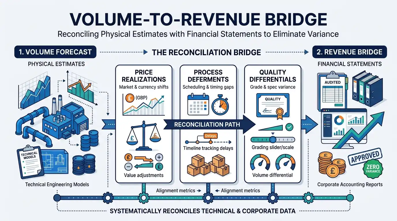
A volume forecast to revenue bridge systematically reconciles physical production estimates with final financial statements by accounting for price realizations, process deferments, and quality differentials. This structured workflow eliminates variance between technical engineering models and corporate accounting reports.

1. Establish the Unconstrained Technical Baseline

The process begins by extracting raw decline curve estimates for every producing well. Reservoir engineers aggregate individual well declines into field-level production profiles using exponential or hyperbolic algorithms. This step establishes theoretical asset capability assuming zero operational interruptions or surface facility bottlenecks.

2. Apply Downtime and Deferment Assumptions

Unconstrained forecasts overestimate real-world production volumes. Corporate planners must adjust the technical baseline by applying historical downtime metrics, scheduled maintenance outages, and seasonal weather disruptions. Deducting these deferment percentages converts theoretical yield into operational volume.

3. Factor In Hydrocarbon Stream Allocations

Raw wellhead production differs significantly from sales-quality gas and liquids. The reconciliation model applies shrinkage factors, fuel gas deductions, and natural gas liquids extraction yields. Converting wellhead fluids into marketable sales units ensures product-level accuracy before financial conversion.

4. Apply Price Realizations and Differential Deductions

Sales volumes are multiplied by benchmark commodity prices, adjusted for regional pricing differentials, energy content, and transportation tariffs. Applying these market-specific adjustments yields the net realized revenue projection, completing the bridge from subsurface volume to financial capital.

How Do Downtime and Deferment Assumptions Reduce Budget Variance?

Factoring historical downtime and planned deferment assumptions into production schedules prevents structural over-forecasting and aligns financial projections with real-world operating conditions. Systematic deferment tracking categorizes planned maintenance, facility bottlenecks, and third-party midstream outages to build defensive cash flow models.

Production facilities operate below theoretical capacity due to equipment degradation, well intervention schedules, and pipeline pressure constraints. Failing to model these operational realities creates systemic upward forecast bias. Financial budgets built on zero-downtime assumptions suffer recurring negative variances throughout the fiscal period.

Operational teams classify deferments into two main categories:

• Planned Deferments: Scheduled turnarounds, regulatory inspections, compressor overhauls, and workover operations.

• Unplanned Deferments: Equipment trips, line relief events, power outages, and adverse weather disruptions.

Analyzing historical mean time between failures provides an empirical base for unplanned loss calculations. Incorporating these statistics directly into rolling forecast schedules ensures cash flow projections withstand unexpected operational downtime.

Establishing structured downtime tracking protocols allows corporate planning units to evaluate the financial impacts of maintenance strategies. Asset managers can model the return on investment of installing backup compression or expanding surface separation capacity. Quantifying deferments transforms maintenance decisions into strategic value drivers.

Why Is Reserves to Production Alignment Essential for Financial Reporting?

Reserves to production alignment ensures that short-term operating budgets mirror long-term reserve replacement strategies, satisfying external regulatory frameworks and internal audit controls. Aligning operational decline estimates with audited reserves figures prevents compliance discrepancies and stabilizes corporate valuation.

Corporate valuations depend on the consistency between publicly reported reserves and annual operational budgets. Discrepancies between SEC-proved reserves and internal production forecasts invite regulatory scrutiny and damage investor confidence. Regular alignment audits ensure short-term operational targets derive directly from audited reserve categories.

Proved Developed Producing reserves form the foundational baseline for immediate operating budgets. Proved Undeveloped and Unproved categories require capital allocation before contributing to production streams. Corporate planners must track conversion timelines to prevent capital misallocation on unverified assets.

Workover campaigns and infill drilling projects shift assets from undeveloped to producing status. Tracking this movement requires continuous communication between subsurface engineers and finance teams. Systematized reserve-to-production reconciliation stops organizations from double-counting volumes or budgeting for delayed projects.

How Does Infill and Workover Uplift Factor Into Capital Budgeting?

Infill drilling and workover uplift provide discrete volumetric additions that offset natural field decline, requiring strict economic gate-keeping before capital inclusion. Financial models must isolate incremental volumes from base field production to evaluate capital efficiency accurately.

Workover interventions—such as re-fracturing, zone completions, and artificial lift optimization—alter the underlying decline mechanics of individual wells. Infill drilling increases total reservoir drainage by accessing previously uncontacted hydrocarbon compartments. Budget models must isolate these high-cost incremental volumes from the base decline profile.

Capital budgeting teams evaluate proposed interventions by comparing capital expenditure against net present value gains. Every workover candidate undergoes incremental rate-of-return analysis based on post-intervention decline forecasts. Unverified uplift projections distort return metrics and risk misallocating corporate funds.

Measuring workover success requires tracking post-project production against original uplift models. Variance analysis isolates technical performance failures from reservoir depletion. Establishing strict baseline accounting ensures that capital-intensive field interventions deliver clear economic additions to corporate revenues.

What Is the Role of Forecast Accuracy Tracking and Bias Analysis in Continuous Improvement?

Forecast accuracy tracking identifies systematic errors in volumetric assumptions, while forecast bias analysis reveals whether planning teams consistently over- or under-estimate production metrics. Systematic variance tracking refines engineering workflows and eliminates corporate risk tolerance drift.

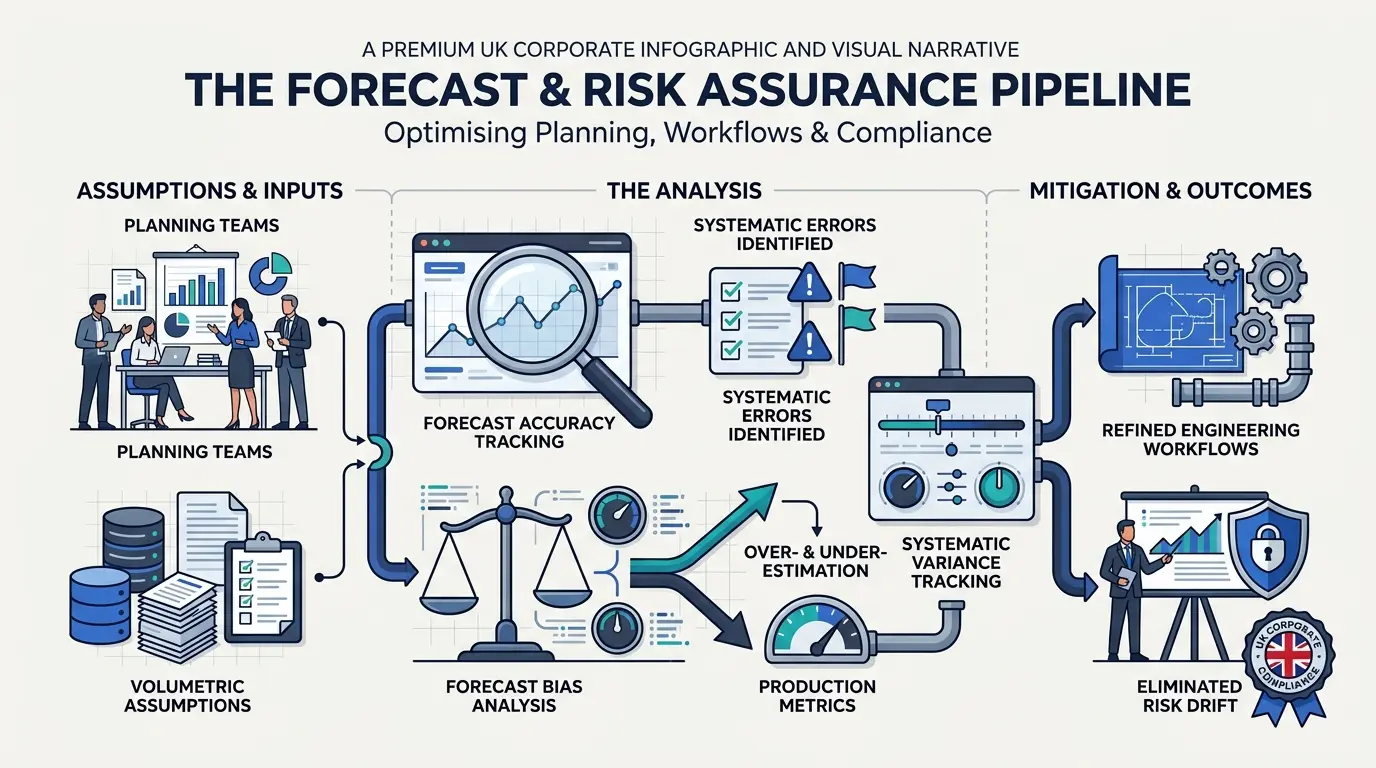
Continuous improvement in financial planning requires tracking production volume accuracy across multiple timeframes. Variance analysis compares actual delivered volumes against baseline projections, isolating operational breakdowns from subsurface modeling errors. Recording these performance metrics establishes clear benchmarks for future planning cycles.

Forecast bias analysis measures the directionality of forecasting errors over long periods. A consistent positive bias indicates over-optimistic engineering assumptions or unmodeled deferments. A consistent negative bias reflects overly conservative planning that starves viable assets of required growth capital.

Eliminating systematic bias requires institutionalizing post-mortem reviews on completed operational quarters. Engineering and finance teams analyze variance root causes to update decline exponents, downtime factors, and workover yield assumptions. This iterative feedback loop continuously recalibrates financial models against field realities.

How Does Rolling Volume Reforecasting Support Dynamic Capital Allocation?

Rolling volume reforecasting replaces static annual plans with continuously updated volumetric projections, allowing corporate leadership to adjust capital allocation as market conditions shift. Updating decline curves quarterly ensures capital expenditure decisions reflect current commodity prices and operational capacity.

Annual static budgets become obsolete when commodity prices fluctuate or key operational milestones shift. Rolling reforecasts integrate updated well tests, new completion data, and revised workover schedules into financial planning models. This fluid visibility protects corporate liquidity during periods of market volatility.

Dynamic capital allocation relies on updated decline curves across all active operating regions. Asset managers reallocate capital from underperforming wells to high-yield intervention opportunities based on quarterly forecast metrics. Rapid capital mobility maximizes return on capital employed across the enterprise portfolio.

Implementing a rolling reforecast process requires integrated financial and engineering software architecture. Unifying subsurface database records with enterprise resource management systems streamlines volumetric data flows. Eliminating manual data transfers reduces human error and accelerates corporate decision-making cycles.

Comparing Workforce Development Approaches for Budgeting Accuracy

Building an accurate petroleum budgeting system requires selecting the right professional development framework for corporate planning teams. Organizations evaluate several capability-building methods to bridge the gap between subsurface technical engineering and financial management.

When evaluating workforce development frameworks, corporate decision-makers must select solutions that target their specific operational capability gaps. Organizations seeking to align engineering decline modeling directly with corporate financial planning often invest in structured external programs, such as specialized Production Forecasting and Decline Curve Analysis Training for Oil and Gas Budgeting Professionals.

Selecting an appropriate learning path depends on corporate organizational maturity, internal engineering capabilities, and financial accuracy targets.

For teams looking to standardize their technical workflows and eliminate forecast bias across planning cycles, the Production Forecasting & Decline Curve Analysis for Budgeting Training Course offers targeted corporate learning models built specifically for oil and gas finance professionals, asset managers, and reservoir engineers.

How to Select the Ideal Petroleum Training Framework for Corporate HR Teams

Selecting an ideal petroleum training framework requires HR leaders to assess current technical skill gaps, evaluate practical delivery models, and demand measurable performance improvements. Effective corporate learning solutions combine subsurface analytical methods with real-world financial management applications.

Evaluating training frameworks requires analyzing how effectively course content bridges cross-functional communication gaps between engineering and finance units. Programs must move beyond theoretical mathematics to address enterprise workflow integration, volumetric reconciliation, and audit compliance metrics.

HR decision-makers should evaluate training options using three core decision criteria:

1. Practical Technical Relevance: Ensure the curriculum covers modern hyperbolic decline mechanics, automated curve fitting, and reserve alignment standards.

2. Cross-Functional Financial Alignment: Confirm that the program directly connects physical volume outputs to revenue conversion workflows, accounting standards, and deferment calculations.

3. Measurable Business ROI: Select providers that measure success through post-training performance improvements, reduced forecast variance, and improved capital allocation efficiency.

Investing in structured team capabilities establishes a standardized forecasting culture across the entire asset portfolio. Aligning technical precision with corporate financial planning minimizes capital risk, improves regulatory compliance, and delivers predictable business outcomes year after year.

Frequently Asked Questions

What does Oil and Gas Petroleum Financial Analysis involve?

Oil and Gas Petroleum Financial Analysis evaluates the commercial viability, fiscal terms, and cash flow dynamics of upstream, midstream, and downstream energy projects. At the Institute For Oil & Gas Training, this analytical process covers net present value (NPV) modeling, capital expenditure (CAPEX) tracking, sensitivity modeling, and risk assessment across changing commodity price environments. Financial analysts use these quantitative techniques to support corporate valuation, capital allocation, and strategic decision-making.

Why is specialized financial analysis important for petroleum industry professionals?

Standard financial models often fail to capture unique energy sector risks such as operational deferments, decline curve dynamics, production-sharing contracts (PSCs), and price volatility. Specialized training through the Institute For Oil & Gas Training equips corporate teams with the skills to translate complex subsurface reservoir data into reliable cash flow projections and financial reports. This specialized knowledge directly improves petroleum budget accuracy and ensures alignment with international financial reporting standards.

How does financial modeling improve budget accuracy in oil and gas companies?

Financial modeling bridges physical production volume forecasts with corporate revenue projections by accounting for operating expenses, price differentials, taxation, and field decline rates. Professionals trained in Oil and Gas Petroleum Financial Analysis at the Institute For Oil & Gas Training learn to build dynamic models that incorporate rolling reforecasts and scenario testing. This systematic approach reduces forecast bias, controls cost variance, and optimizes long-term capital allocation strategies.

Who should undertake training in Oil and Gas Petroleum Financial Analysis?

This specialized training is designed for corporate planning managers, finance professionals, commercial analysts, reservoir engineers, and HR teams seeking to bridge technical and financial skills gaps within their organisations. The Institute For Oil & Gas Training delivers practical, industry-aligned instruction that enables cross-functional teams to evaluate asset performance collaboratively. Participants gain actionable expertise in capital budgeting, project evaluation, and energy corporate finance.

What key financial metrics are used to evaluate petroleum assets?

Petroleum asset evaluation relies on metrics such as Net Present Value (NPV), Internal Rate of Return (IRR), Payback Period, Finding and Development (F&D) costs, and Earnings Before Interest, Tax, Depreciation, and Amortisation (EBITDA). The Oil and Gas Petroleum Financial Analysis program at the Institute For Oil & Gas Training teaches professionals how to calculate and stress-test these metrics against various fiscal regimes and market conditions to maximize asset portfolio value.